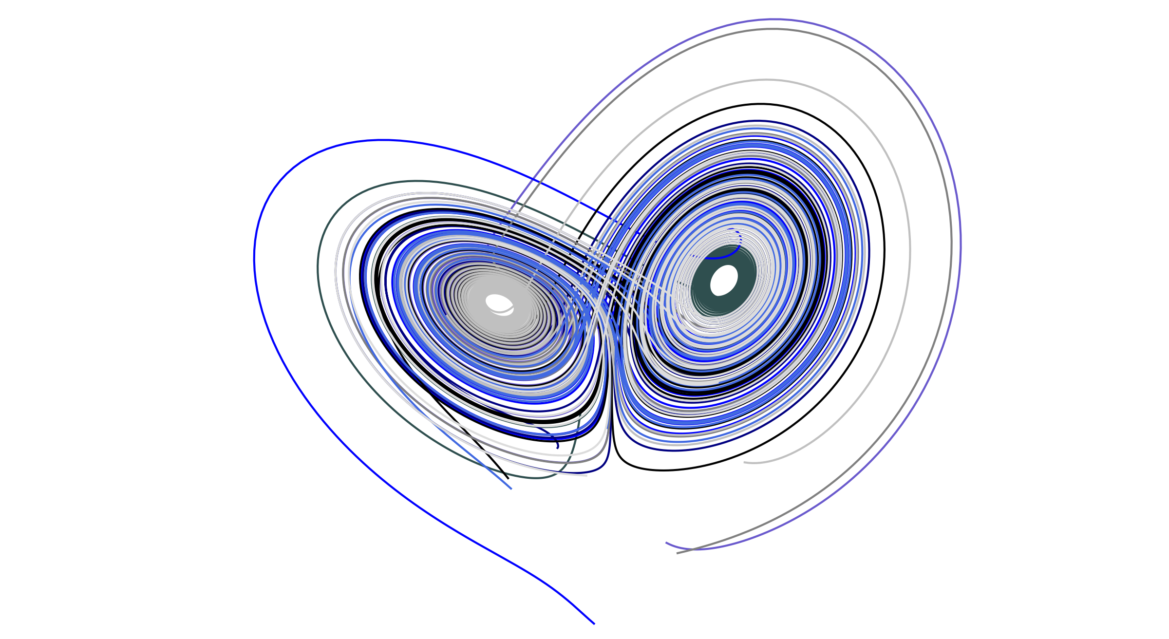
Visualization of Cool Attractors
Contents
In case you liked the attractor in my About Me page, this code will generate the same plot. We will be using only the libraries numpy, matplotlib and scipy in Python, but Plots and Differential Equations in Julia. I learned these skills thanks to this cool article by Jake VanderPlas. I am interested in exploring many chaotic systems, so this post will try to address some other cool attractors. All examples here are written in Python. The Julia code will be available at the end of each section.
import numpy as np
from scipy.integrate import odeint
from matplotlib import pyplot as plt
The Lorenz Attractor

This one is so cool that does not need introduction, son lets get coding. Now we declare a function to compute de Lorenz system of differential equations. The parameters $\sigma$, $\beta$ and $\rho$ are given directly. The function is designed to input a point in $\mathbb{R}^3$ and return the derivatives of each variable.
def lorenz(state, t, sigma=10.0, beta=8.0/3.0, rho=28.0):
    x, y, z = state
    dx = sigma * (y - x)
    dy = x * (rho - z) - y
    dz = x * y - beta * z
    return [dx, dy, dz]
We are going to solve the Lorenz system for 9 initial conditions. We want the butterfly shape to have many colors, and that is why we use one color for each solution curve. All initial conditions will be random numbers between -15 and 15. We use a seed for the np.random.random function so the graphics are the same allways. The simulation time will be of 20 units of time, using 8000 points. Solutions to Lorenz are stored in a three dimensional array. We use a list comprehention to avoid excesive notation.
np.random.seed(10)   # Try these, they are very cool: 6, 7, 10*, 15
N   = 9
x0  = -15 + 30 * np.random.random((N, 3))
t   = np.linspace(0, 20, 8000)
xt  = np.asarray([odeint(lorenz, i, t) for i in x0])
Results will be ploted in a 3D projection using matplotlib. The figure object contains one matplotlib.axis. All 9 solution curves will be on the same phase space. We turn off the axis so we only wet the interesting part of the plot. We define the limits of the plot too.
fig = plt.figure(figsize=(12, 12))
ax  = fig.add_subplot(1, 1, 1, projection='3d')
ax.axis('off')
ax.set_xlim((-25, 25))
ax.set_ylim((-35, 35))
ax.set_zlim((5, 55))
All collors supported by matplotlib can be found here. Those used for our plot are in the colors list. Using a for loop we plot all sets of points in the solution array. We pick the colors for each curve in order. Finally, we set the angles at which we see the 3D plot using the ax.view_init function. Then we save a transparent image so it can fit on any backgroud.
colors = ['darkslategray', 'slateblue', 'blue', 'navy', 'black', 'gray',
          'silver','royalblue','gainsboro']

for i in range(N):
    ax.plot3D(xt[i,:,0], xt[i,:,1], xt[i,:,2], colors[i])

ax.view_init(-25, -40)
name = "lorenz_attractor.png"
plt.savefig(name, transparent=True, dpi=300, bbox_inches=0.0, pad_inches=0.0)
plt.show()